 1999, First-Grade Homework")

Preface:
Upon reading chapter four of my assigned physics textbook [Modern Physics, Krane], I grew both tired and annoyed with the generalizations, or “leaps of faith” which author continually made. I soon found it more useful instead, to spend time reading the papers upon which these principals have been derived. Astonishingly however, I failed to find a modern, usable English translation of Werner Heisenberg’s landmark paper! More unfortunately even, the closest I did come on the hunt for such a translation was the discovery of a broken-english, NASA OCR script from 1988 hosted on the web archive. That won’t do.
Thus utilizing a day’s time, Google translate, MathJax and my personal skills at reading broken-english datasheets, I below have provided a modern translation of W. Heisenberg’s paper. For convenience of the reader, I have replaced some original variables used in the paper to more represent those found in common texts today. New notations such as euclidean norms (i.e, \(|f(x)|\)) have been instated, as well.
Dr. Heisenberg’s various justifications alone make for an interesting (and perhaps, very useful!) read, but for those short on time I have prepared also, a “too long, didn’t read” summary immediately preceding.
TLDR Summary
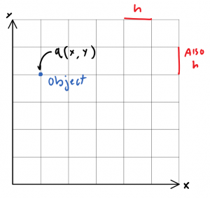 If we are to derive a model that quantizes space, perhaps to cells with lengths some finite dimension \(h\), then we are left with in the space \(\mathbb{Q}^2\) for example, a 2-dimensional grid of possible positions. Objects in this grid then, may be given some arbitrarily-defined co-ordinate, \(q\).
q of course, is a function of \((x,y)\) inside \(\mathbb{Q}^2\). \(x\), and \(y\) may only be integer multiples of h, or specifically:
\(q = \left \{ \forall (x, y)*h\in\mathbb{Q}^2 \right \}\)(don’t be scared, I’m just having fun with LaTeX!)
 Now, if \(q\) is a function of yet another quantized variable, \(t\), then \(q(x,y)\) may be broken into \(q(x(t),y(t))\).
Thus if it’s fair to say “\(q\) can move as time advances integer multiples of h”, then it is possible to define some distance \(q_x\), that \(q\) has moved in that elapsed time \(\Delta t\). We may thus define a 1-dimensional “velocity” \(v_x = \frac{\Delta q_x}{\Delta t}\).
\(q\) however, is not a continuous function in this space, as it may only take on discrete values, themselves integer multiples of \(h\). Therefore it is useless to define “the velocity at a point”. More generally, \(q\)‘s average velocity for any time interval, \(\Delta t\), smaller than \(h\), is not definable.
Restated, only values of \(q_x\), or \(v_x\), can satisfy the below statement;
If time advances as \((integers) * h\), then \(\Delta q_x \geq h\) if our definition of “velocity” is to make any sense.
By extension, momentum in this direction, which is defined as \(m v_x\) must satisfy \(p_x \geq h\), if \(m\) can be no smaller than \(h\) as well.
Now consider the thought:
What if we were to look at the object \(q\), with absolute precision? That is, \(q_x\) is exactly defined, and \(\Delta q_x = 0\).
Then, if \(v_x\) is a function of \(\Delta q_x\) then as \(\Delta q_x(t \rightarrow 0)\), or “the change in \(q_x\)” approaches zero, then the function \(v_x(\Delta q_x(t \rightarrow 0))\) becomes indeterminate. This relation works on the converse as well, such that the relation:
\(\Delta q_x * m \Delta v_x \geq h\) is justified!
In our 3 dimensional world \(\mathbb{Q}^3\), this equation becomes the familiar Heisenberg uncertainty principal:
\(\Delta q_x\;\Delta p_x \geq \frac{h}{2 \pi}\)The factor of \(2 \pi\) is a geometric normalization.
The origins of this relation’s elegance are plain to see: it is one derived from simple principals! Below, Heisenberg purports similar arguments exist for an energy-time relationship, and proves both relations are just as true for wave-functions as they are for discrete, “particle” functions. I’ll leave that lesson to be a test of your reading comprehension skills, however.
Über den inhalt der quantentheoretischen anschaulichen the kinematik und mechanik (or, the actual content of quantum theoretical kinematics and mechanics)
W. Heisenberg, a modern translation by Adam Munich
First, exact definitions are supplied in this paper for the terms: position, velocity, energy, etc. (of the electron, for instance), such that they are valid also in quantum mechanics; then we shall show that canonically conjugated variables can be determined simultaneously only with a characteristic uncertainty. This uncertainty is the intrinsic reason for the occurrence of statistical relations in quantum mechanics. Their mathematical formulation is made possible by the Dirac-Jordan theory. Beginning from the basic principles thus obtained, we shall show how macroscopic processes can be understood from the viewpoint of quantum mechanics. Several imaginary experiments are discussed to elucidate the theory.
We believe to understand a theory intuitively, if in all simple cases we can qualitatively imagine the theory’s experimental consequences and if we have simultaneously realized that the application of the theory excludes internal contradictions. For instance: we believe to understand Einstein’s concept of a finite three-dimensional space intuitively, because we can Imagine the experimental consequences of this concept without contradictions. Of course, these consequences contradict our customary intuitive space-time beliefs. But we can convince ourselves that the possibility of applying this customary view of space and time can not be deduced either from our laws of thinking, or from experience.
The intuitive interpretation of quantum mechanics is still full of internal contradictions, which become apparent in the battle of opinions on the theory of continuums and discontinuums, particles and waves. This alone tempts us to believe that an interpretation of quantum mechanics is not going to be possible in the customary terms of kinematic and mechanical concepts. Quantum theory, after, derives from the attempt to break with those customary concepts of kinematics and replace them with relations between concrete, experimentally derived values. Since this appears to have succeeded, the mathematical structure of quantum mechanics won’t require revision, on the other hand. By the same token, a revision of the space-time geometry for small spaces and times will also not be necessary, since by a choice of arbitrarily heavy masses the laws of quantum mechanics can be made to approach the classic laws as closely as desired, no matter how small the spaces and times. The fact that a revision of the kinematic and mechanic concepts is required seems to follow immediately from the basic equations of quantum mechanics.
Given a mass \(m\), it is readily understandable, in our customary understanding, to speak of the position and of the velocity of the center of gravity of that mass \(m\). But in quantum mechanics, a relation \( \mathbf{p\;q-q\;p} = \frac{h}{2 \pi} \) exists between mass, position and velocity. We thus have good reasons to suspect the uncritical application of the terms “position” and “velocity”. If we admit that for very small spaces and times discontinuities are somehow typical, then the failure of the concepts precisely of “position” and “velocity” become immediately plausible:
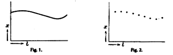
If, for instance, we imagine the one-dimensional motion of a mass point, then in a continuum theory it will be possible to trace the trajectory curve \(x(t)\) for the particle’s trajectory (or rather, that of its center of mass) [see Fig. l, above], with the tangent vector to the curve indicating the velocity, in each case.
In a discontinuous theory, in contrast, instead of a smooth curve we shall have a series of points spaced at finite distances [see Fig. 2, above]. In this case it is obviously pointless to talk of the velocity at a certain position, since the velocity can be defined only by means of two positions, with two different velocities corresponding to each point.
The question thus arises whether it might not be possible, by means of a more precise analysis of those kinematic and mechanical concepts, to clear up the contradictions currently existing in an intuitive interpretation of quantum mechanics, to thus achieve an intuitive understanding of the relations of quantum mechanics.1
1 This paper was written as a consequence of the efforts and wishes expressed clearly by other scientists much earlier, before quantum mechanics was developed. I particularly remember Bohr’s papers on the basic tenets of quantum theory (for instance, Z.f. Physik 13, 117 (1923)) and Einstein’s discussions on the relation between wave fields and light quanta. In more recent times, the problems here mentioned were discussed most clearly by W. Pauli, who also answered some of the questions that arise (“Quantentheorie, Handbuch d.Phys. [“Quantum theory”, Handbook of Physics] Vol. XXIII). Quantum mechanics has changed little in the formulation Pauli gave to these problems. It is also a special pleasure for me here to thank Mr. W. Pauli for the stimulation I derived from our oral and written discussions, which have substantially contributed to this paper.
§1, the concepts: position, path, velocity, energy
In order to be able to follow the quantum-mechanical behavior of any object, it is necessary to know the object’s mass and and the interactive forces with any fields or other objects. Only then is it possible to set up the Hamiltonian function for the quantum-mechanical system. I shall in general refer to non-relativistic quantum mechanics, since the laws of quantum-theory electrodynamics are not completely known yet.
If we want to clearly understand what is meant by the word “position of the object” – for instance, an electron relative to a given reference system, then we must indicate the definite experiments by means of which we intend to determine the “position of the electron.” Otherwise the word is meaningless. In principle, there is no shortage of experiments that permit a determination of the “position of the electron” to any desired precision, even. For instance: illuminate the electron and look at it under the microscope. The highest precision attainable here in the determination of the position is substantially determined by the wavelength of the light used.
But let us imagine however a gamma-ray microscope and by means of it, determine the position as precisely as desired. But in this determination a secondary circumstance becomes essential: the Compton effect. Any observation of the scattered light coming from the electron (into the eye, onto a photographic plate, into a photocell) presupposes a photoelectric effect. That is, this event may also be interpreted as a photon striking the electron, there being reflected or diffracted to then deflected once again by the microscope’s lens, finally triggering the photoelectric effect.
At the instant of the determination of its position – in example, the instant at which the photon is diffracted by the electron, the electron discontinuously changes its impulse. That change will be more pronounced the smaller the wavelength of the light used, i.e, the more precise the position determination is to be. In the instant at which the electron’s position is known, therefore, its impulse can become known only to the nearest order of magnitude corresponding to that discontinuous change. That is, the more precisely the position is determined, the more imprecisely the impulse will be known, and vice-versa. This provides us with a direct, intuitive clarification of the relation \( \mathbf{p\;q-q\;p} = \frac{h}{2 \pi} \).
Let \(\Delta q\) be the precision to which the value of \(q\) is known (\(\Delta q\) is approximately the average error of \(q_1\)), or here, the wavelength of the light used to “see” the object. Let \(\Delta p\) be the precision to which the value of \(p\), the object’s momentum, can be determined, or in this case, the discontinuous change in \(p\) during the Compton effect. According to the basic equations of the Compton effect, the relation between \(\Delta q\) and \(\Delta p\) is then:
How that relation (1) above stands in a direct mathematical connection with the commutation relation \(\mathbf{pq-qp} = \frac{\hbar}{2 \pi}\) shall be shown below. Here we shall point out that equation (1) is the precise expression for the fact that we once sought to describe by dividing the phase space into cells of size \(h\).
Other experiments can also be performed to determine the electron’s position, such as impact tests. A very precise determination of the position requires impacts with very fast particles, since for slow electrons the diffraction phenomena, which according to Einstein are a consequence of the de Broglie waves (see for instance the Ramsay effect), preclude a precise determination of the position. Thus, once again for a precise position measurement the electron’s impulse changes discontinuously and a simple estimate of the precision with the equations of the de Broglie waves once again leads to equation (1).
This discussion seems to define the concept of position of the electron clearly enough and we only need to add a word about the “size” of the electron. If two very fast particles strike the electron sequentially in the very brief time interval \(\Delta t\), then the two positions of the electron defined by these two particles lie very close together, separated by a distance \(\Delta l\). From the laws observed for alpha-particles we conclude that \(\Delta l\) can be reduced to a magnitude of the order of \(10^{-12}\) cm, provided \(\Delta t\) is sufficiently small and the particles selected are sufficiently fast. That is the meaning, when we say that the electron is a particle whose radius is not greater than \(10^{-12}\) cm.
Let us move on to the concept of the “path of the electron.” By path or trajectory we mean a series of points in space (in a given reference system) that the electron adopts as successive “positions.” Since we already know what “position at a certain time” means, there are no new difficulties here. It is still readily understood that the often used expression, for instance, “the 1s orbit of the electron in the hydrogen atom” makes no sense, from out point of view. Because in order to measure this 1s orbit, we would have to illuminate the atom with light such that its wavelength is considerably shorter than its “size”, approximately \(10^{-8}\) cm.
But one light quantum of this kind of light would be sufficient to completely throw the electron out of its “orbit” (for which reason never more than a single point of this “path” could be defined, in space) and hence the word “path” is not very sensible or meaningful, here. This can be easily derived from the experimental possibilities, even without any knowledge of the new theories.
In contrast, the imaginary position measurements can be performed for many atoms in a 1s state. (Atoms in a given “stationary” state, for instance, can in principle be isolated by the Stern-Gerlach experiment) Thus, for a given state, for instance 1s, of an atom, a probability function must exist for the electron’s positions, such that it corresponds on the average, to the classical trajectory over all phases, and that can be established by measurements to any desired precision.
According to Born2 this function is given by \(|\psi _{1s}(x)|^2\), where \(\psi _{1s}(x)\) is the Schroedinger wave function corresponding to the state 1s. I want to join Dirac and Jordan, in view of subsequent generalizations, in saying: the probability is given by \(|S(1s, q)|^2\), where \(S(1s, q)\) is that column of the transformation matrix \(S\) from \(E\) to \(q\), which corresponds to \(E = E_{1s}\) ( where \(E\) = Energy)
2 The statistical meaning of the de Broglie waves was first formulated by A. Einstein [Sitzungsber.d.preuss.Akad.d.Wiss. 1925, p3]. This statistical element then plays a significant role for M. Born, W. Heisenberg and P. Jordan, [“Quantum mechanics 11.” [Z.f.Phys. 35, 557 (1926)], especially chapter 4, 53, and P. Jordan” TZ. .Phys, 37, 376
(1926)]; it is analyzed mathematically in a fundamental paper by M. Born [Z.f.Phys. 38, 803 (1926)] and used for the interpretation of the collision phenomena. The foundation for using the probability theorem from the transformation theory for matrices can be found in: [W. Heisenberg (Z. f.Phys. AO, 501 (1926)], P. Jordan [libid. 40, 661 (1926)], W. Pauli. [in Z.f.Phys. 41, 81 (1927)] P. Dirac [Proc. Roy, Soc.(A) U2f 621 (1926)], P. Jordan [Z.f.Phys. 40, 809 (1926)]. The statistical side of quantum mechanics in general is discussed by P. Jordan [Naturwiss. 15, 105 (1927)] and M. Born [Naturwiss. 15, 238 (1927)].
In the fact that in quantum theory for a given state, for instance 1s – only the probability function for the electron position can be given, we may see a characteristic statistical feature of quantum theory, as do Born and Jordan, quite in contrast to the classical theory. On the other hand, if we want to we can say with Dirac that the statistics came in via our experiments. Because also in classical theory only the probability of a certain electron position could be given, as long as we do not know the atom’s phases. Rather, the difference between classical and quantum mechanics consists in this: classically, we can always assume the phases to have been determined in a previous experiment. But in reality this is impossible, because every experiment to determine the phase would either destroy or modify the atom. In a definite stationary “state” of the atom, the phases are indeterminate in principle, which we may consider a direct clarification of the
known equations:
Where \(\mathbf{J}\) is the action variable and \(\mathbf{\omega}\) is the angular variable.
The word “velocity” of an object is easily defined by measurement if it is a force-free motion. For instance, the object can be illuminated with red light and then the particle’s velocity can be determined by the Doppler effect of the scattered light. The determination of the velocity will be the more precise, the longer the wavelength of the light used is, since then the particle’s velocity change per incident photon due to the Compton effect will be the smaller. The position determination becomes correspondingly uncertain, as required by equation (1). If the velocity of the electron in an atom is to be measured at a certain instant, we should have to make the nuclear charge and the forces due to the other electrons disappear, at that instant, so that the motion may proceed force free, after that instant, to then perform the determination described above.
As was the case earlier, we once again can convince ourselves that a function \(p(t)\) for a certain state of the atom – say, 1s – can not be defined. In contrast, there again will be a function for the probability of \(p\); this state, which according to Dirac and Jordan will have the value \(|S(1s, \mathbf{p})|^2\). Again, \(S(1S, p)\) means the column of the transformation matrix \(S\) of \(E\) into \(p\) that corresponds to \(E=E_{1S}\).
Finally, let us point out the experiments that allow the measurement of the energy or the value of the action variables \(\mathbf{J}\). Such experiments are particularly important since only with their aid will we be able to define what we mean, when we talk about the discontinuous change of the energy of \(\mathbf{J}\). The Franck-Hertz collision experiments permit the tracing back of the energy measurements on atoms to the energy measurements of electrons moving in a straight line, because of the validity of the energy theorem in the quantum theory.
In principle, this measurement can be made as precise as desired if we forego the simultaneous determination of the electron position, i.e., of the phase (see above, the determination of p), corresponding to the relation \( \mathbf{Et-tE} = \frac{h}{2 \pi i} \). The Stern-Gerlach experiment permits the determination of the magnetic or an average electric moment of the atom, i.e., the measurement of magnitudes that depend only the action variables \(\mathbf{J}\). The phases remain undetermined in principle. If it is not sensible to talk of the frequency of a light wave at a given instant, it is not possible either to speak of the energy of an atom at a particular instant.
In the Stern-Gerlach experiment this corresponds to the situation that the precision of the energy measurement will be the smaller, the shorter the time interval during which the atom is under the influence of the deflecting force. Because an upper limit for the deflecting force is given by the fact that the potential energy of that deflecting force inside the beam of rays can vary only by quantities that are considerably smaller than the energy differences of the stationary states, if a determination of the stationary states’ energy is to be possible. If \(\Delta E\) is the quantity of energy that satisfies that condition, (\(\Delta E\) at the same time is a measure of the precision of that energy measurement), then \(\frac{\Delta E}{d}\) is the maximum value for the deflecting force, if d is the width of the ray beam (measurable by means of the width of the slit used).
The angular deflection of the atom beam is then \(\frac{\Delta E \Delta t}{d \Delta p}\) where \(\Delta t\) is the period of time during which the atoms are under the effect of the deflecting force, \(\Delta p\) is the impulse of the atoms in the direction of the beam. This deflection must be at least of the same order of magnitude as the natural beam broadening caused by diffraction in the slit, in order for a measurement to be possible. The angular deflection due to diffraction is approximately \(\frac{\lambda}{d}\), where \(\lambda\) is the de Broglie wavelength, i.e…
\(\frac{\lambda}{d} \sim \frac{\Delta E \Delta t}{d \Delta p}\) and since \(\lambda = \frac{h}{p}\)
This equation corresponds to equation (1) and it shows that a precise energy determination can be attained only through a corresponding uncertainty in the time.
§2, the Dirac-Jordan theory
We would like to summarize the results of the previous section and generalize them in this statement: all concepts used in classical theory to describe a mechanical system can also be defined exactly for atomic processes, in analogy to the classic concepts. But purely from experimentation, the experiments that serve for such definitions carry an inherent uncertainty, if we expect from them the simultaneous determination of two canonically conjugated variables. The degree of this uncertainty is given by equation (1), widened to include any canonically conjugated variables. It is reasonable then, to compare the quantum theory with the special theory of relativity.
According to the theory of relativity, the term “simultaneous” can only be defined by experiments in which the propagation velocity of light plays an essential role. If there were a “sharper” definition of simultaneity – for instance, signals that propagate infinitely rapidly – then the theory of relativity would be impossible. But since such signals do not exist – because the velocity of light already appears in the definition of simultaneity – room is available for the postulate of a constant velocity of light and therefore this postulate is not contradicted by the appropriate use of the terms “position, velocity, time”.
The situation is similar in regard to the definition of the concepts “electron position” and “velocity”, in quantum theory. All the experiments we could use to define these terms necessarily contain the uncertainty expressed by equation (1), even though they permit an exact definition of the individual concepts \(\Delta p\) and \(\Delta q\). If experiments existed that allowed a “more precise” definition of \(\Delta p\) and \(\Delta q\) than that corresponding to equation (1), then quantum theory would be impossible.
This uncertainty – which is fixed by equation (1)
Now provides the space for the relations that find terse expression in the commutation relations of quantum mechanics. This equation becomes possible without having to change the physical meaning of the differences, \(\Delta p\) and \(\Delta q\).
For those physical phenomena for which a quantum theory formulation is still unknown (for instance, electrodynamics), equation (1) represents a demand that may be helpful in finding the new laws. For quantum mechanics, equation (1) can be derived from the Dirac-Jordan formulation, by means of a minor generalization. If for a certain value of an arbitrary parameter \(\eta\) we can determine the position \(q\) of the electron at \(q’\) with a precision \(\Delta q\), then we can express this fact by means of a probability density \(\psi(\eta, q)\) that will be noticeably different from zero only in an area of approximate dimension \(\Delta q\) around \(q’\). We can thus say, more specifically:
We thus have for the probability amplitude corresponding to \(p\):
In agreement with Jordan, we can say:
In that case, according to (4), \(S(\eta,p)\) will be noticeably different from zero only for values of \(p\) for which \(\frac{2 \pi (p – p’) \Delta q}{h}\) is not substantially larger than 1. More especially, in the case of (3) we shall have:
Thus, assumption (3) for \(S(\eta,p)\) corresponds to the experimental fact that the value \(p’\) of \(p\) and the value \(q’\) of \(q\) were measured [with the precision restriction (6)].
The purely mathematical characteristic of the Dirac-Jordan formulation of quantum mechanics is that the relations between \(\mathbf{p, q}, E\), etc., can be written as equations between very general matrices, such that any variable indicated by quantum theory appears as the diagonal matrix. The feasibility of such a notation seem reasonable if we visualize the matrices as tensors (for instance, moments of inertia) in multidimensional spaces, among which mathematical relations exist. The axes of the coordinate system in which these mathematical relations are expressed can always be placed along the main axis of one of these tensors. It is after all always possible to characterize the mathematical relation between two tensors \(\mathbf{A}\) and \(\mathbf{B}\) by means of transformation formulae that will convert a system of coordinates oriented along the main axis of \(\mathbf{A}\), into one oriented along the main axis of \(\mathbf{B}\). The latter formulation corresponds to Schroedinger’s theory.
In contrast, Dirac’s notation of the q-numbers must be considered the truly “invariant” formulation of quantum mechanics, independent of all coordinate systems. If we wanted to derive physical results from that mathematical model, then we must assign numerical values to the quantum mechanics variables, i.e., the matrices (or “tensors” in multidimensional space). This is to be understood as meaning that in that multidimensional space a certain direction is arbitrarily chosen (that is, established by the kind of experiment performed), and then the “value” of the matrix is asked for (for instance, the value of the moment of inertia, in that picture), in the direction chosen. This question has unequivocal meaning only if the direction chosen coincides with one of the matrix’s main axes: in that case there will be an exact answer to the question. If the direction chosen deviates but little from one of the matrix’s main directions, we can still talk with a certain imprecision, given by the relative inclination, with a certain probable error of the “value” of the matrix in the direction chosen.
We can thus state: it is possible to assign a number to every quantum theory variable, or matrix, which provides its “value”, with a certain probable error. The probable error depends on the system of coordinates. For each quantum mechanics variable there exists one system of coordinates for which the probable error vanishes for that variable. Thus, a given experiment can never provide precise information on all quantum mechanics variables: rather, it divides the physical variables into “known” and “unknown” (or: more or less precisely known variables), in a manner characteristic for that experiment. The results of two experiments can be derived precisely from each other only when the two experiments divide the physical variables in the same manner into “known” and “unknown” (i,e., if the tensors in that multidimensional space already used for visualization are viewed from the same direction, in both experiments.) If two experiments cause two different distributions into “known” and “unknown” variables, then the relation of the results of those experiments can be given appropriately only statistically.
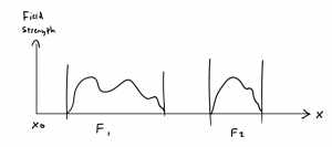
Let us perform an imaginary experiment, to more precisely discuss these statistical relations. We shall start by sending a Stern-Gerlach beam of atoms through a field \(F_1\) that is so heterogeneous in the beam direction, that it causes noticeably numerous transitions due to a “shaking effect”. The atom beam is then allowed to run unimpeded, but then a second field shall begin, \(F_2\), as heterogeneous as \(F_1\). We shall assume that it is possible to measure the number of atoms in the different stationary states, between \(F_1\) and \(F_2\) and also beyond \(F_2\) by means of an eventually applied magnetic field. Let us assume the atoms’ radiative forces to be zero.
If we know that an atom was in the energy state \(E_n\) before passing through \(F_1\), then we can express this experimental fact by assigning a wave function to the atom – for instance, in \(\mathbb{p}\)-space – with a certain energy \(E_n\) – and the undetermined phase \(\phi_n\), and an initial phase \(\phi_0\):
Let us assume that here the \(\phi_n\) are arbitrarily fixed, such that the \(c_{n\;m}\) is unequivocally determined by \(F_1\), The matrix \(c_{n\;m}\) transforms the energy value before passing through \(F_1\) to that after passing through \(F_1\). If behind \(F_1\) we perform a determination of the stationary states – for instance, by means of an heterogeneous magnetic field – then we shall find, with a probability of \(c_{n\;m}\overline{c_{n\;m}}\) that the atom has passed from the state n to the state m. If we determine experimentally that the atom has actually acquired the state m, then in the subsequent calculations we shall have to assign it the function \(\sum_{m}c_{n\;m}S_{m}\) with an indeterminate phase, instead of the function \(S_m\).
Through the experimental determination “state m” we select, from among the different possibilities \(c_{n\;m}\), a certain m and simultaneously destroy, as we shall explain below, whatever remained of phase relations in the variables \(c_{n m}\). When the beam passes through \(F_2\), we repeat the same procedure used for \(F_1\). Let \(d_{n\;m}\) be the coefficients of the transformation matrix that convert the energies before \(F_2\) to those after \(F_2\). If no determination of the state is performed between \(F_1\) and \(F_2\), then the eigenfunction is transformed according to the following pattern:
Let \(\sum_{m}c_{n\;m}d_{m\;l} = e_{n\;l}\). If the stationary state of the atom is determined, after \(F_2\), we shall find the state “l” with a probability of \(e_{nl}\overline{e_{n\;l}}\). If in contrast, we determined “state m” between \(F_1\) and \(F_2\), then the probability for “l” behind \(F_2\) is given by \(d_{n\;l}\overline{d_{n\;l}}\). Repeating the entire experiment several times, (determining the state, each time, between \(F_1\) and \(F_2\)) we shall then observe the state “l”, behind \(F_2\) with the relative frequency \(\sum_{m}c_{n m}\overline{c_{n\;m}}d_{m\;l}\overline{d_{m\;l}}\). This expression does not agree with \(E_{n\;l}\overline{E_{n\;l}}\).
For this reason Jordan mentions an “interference of the probabilities”. I, for one, would not agree with this, because the two experiments leading to \(E_{n\;l}\overline{E_{n\;l}}\) or \(Z_{n\;l}\), respectively, are really physically different. In one case the atom suffers no disturbance between \(F_1\) and \(F_2\). In the other it is disturbed by the equipment that makes the determination of the stationary states possible. The consequence of this equipment is that the “phase” of the atom changes by quantities that are uncontrollable in principle, just as the impulse was changed in the determination of the electron’s position (of. §1). The magnetic field for the determination of the state between \(F_1\) and \(F_2\) will change the eigenvalues \(E\) and during the observation of the atom beam (I am thinking of something like a Wilson track) the atoms will be slowed down in different degrees, statistically, and in an uncontrollable manner. As a consequence, the final transformation matrix \(E_{n\;l}\) (from the energy values before \(F_1\) to those after leaving \(F_2\)) is no longer given by \(\sum_{m}c_{n\;m}d_{m\;l}\), and instead each term of the sum will have, in addition, an unknown phase factor. Hence, all we can expect is for the average value of \(E_{n\;l}\overline{E_{n\;l}}\) over all eventual phase changes, to be equal to \(Z_{n\;l}\). A simple calculation shows this to be the case.
Thus following certain statistical rules, we can draw conclusions, based on one experiment, regarding the results possible for another. The other experiment selects, by itself and from among all the possibilities, one particular one, thus limiting the possibilities for all subsequent experiments. This interpretation of the equation for the transformation matrix \(S\), or Schrodinger’s wave equation, is possible only because the sum of all solutions is also a solution. Here we can see the deeper meaning of the linearity of Schrodinger’s equations and hence they can be understood only as waves in the phase space; for it is same reason we would consider any attempt to replace these equations – for instance, in the relativistic case (for several electrons) – by non-linear equations is doomed to failure.
§3, The transition from micro to macro-mechanics
I believe the analyses performed in the preceding sections of the terms “electron position”, “velocity”, “energy”, et cetera, have sufficiently clarified the concepts of quantum theory kinematics and mechanics, so that an intuitive understanding of the macroscopic processes must also be possible, from the point of view of quantum mechanics. The transition from micro to macro mechanics has already been dealt with by Schrodinger, but I do not believe that Schrodinger’s considerations address the essence of the problem, for the following reasons: according to Schrodinger, in highly excited states a sum of the eigenvibrations will yield a not overly large wave packet, that in its turn, under periodic changes of its size, performs the periodic motions of the classical “electron”. The following objections can be raised here:
If the wave packet had such properties as described here, then the radiation emitted by the atom could be developed into a Fourier series in which the frequencies of the harmonic vibrations are integer multiples of the fundamental frequency. Instead, the frequencies of the spectral lines emitted by the atom are never integer multiples of a fundamental frequency, according to quantum mechanics – with the exception of the special case of the harmonic oscillator. Thus Schrodinger’s consideration is applicable only to the harmonic oscillator considered by him, while in all other cases in the course of time the wave packet spreads over all space surrounding the atom. The higher the atom’s excitation state, the slower will be the scattering of the wave packet. But it will occur, if one waits long enough.
The argument used above for the radiation emitted by an atom can be used, for the time being, against all attempts of a direct transition from quantum to classical mechanics, for high quantum numbers. For this reason, it used to be attempted to circumvent that argument by pointing to the natural beam width of the stationary states; certainly improperly, since in the first place this way out is already blocked for the hydrogen atom, because of insufficient radiation at higher states; in the second place, the transition from quantum to classical mechanics must be understandable without borrowing from electrodynamics. Bohr has repeatedly pointed out these known difficulties, in the past, that make a direct connection between quantum and classical theory difficult. If we explained them here again in such detail, it is because apparently they have been forgotten.
I believe the genesis of the classical “orbit” can be precisely formulated thus: the “orbit” only comes into being by our observing it. Let us assume an atom in its thousandth excitation state. The dimensions of the orbit are relatively large here, already, so that it is sufficient, in the sense of §1, to determine the electron’s position with a light of relatively long wavelength. If the determination of the electron’s position is not to be too uncertain, then one consequence of Compton recoil will be that after the collision, the atom will be in some state between, say, the 950th and the 1050th. At the same time, the electron’s impulse can be derived – to a precision given by equation (1) – from the Doppler effect. The experimental fact so obtained can be characterized by means of a wave packet – or better, probability packet – in \(\mathbb{q}\)-space, by a variable given by the wavelength of the light used, essentially composed of eigenfunctions between the 950th and the 1050th eigenfunction, and through the corresponding packet in \(\mathbb{p}\)-space. After a certain time, a new position determination is performed to the same precision.
According to §2, its result can be expressed only statistically; possible positions are all those within the now already spread wave packet, with a calculable probability. This would in no way be different in classical theory, since in classical theory the result of the second position could also be given only statistically, due to the uncertainty in the first determination; in addition, the system’s orbits would also spread in classical theory similarly to the wave packet. However, the laws of statistics themselves are different in quantum mechanics and classical theory. The second position determination “\(q\)” selected from among all those possible, thus limiting the possibilities for all subsequent determinations. After the second position determination, the results for later measurements can be calculated only by again assigning to the electron a “smaller” wave packet of dimension \(\lambda\) (the wavelength of the light used for the observation).
Thus, each position determination reduces the wave packet again to its original dimension \(\lambda\). The “values” of the variables \(p\) and \(q\) are known to a certain precision, during all experiments. Since within these limits of precision the values of \(p\) and \(q\) follow the classical equations of motion, we can conclude, directly from the laws of quantum mechanics:
But as we mentioned, the orbit can only be calculated statistically from the initial conditions, which we may consider a consequence uncertainty existing in principle, in the initial conditions. The laws of statistics are different for quantum mechanics and classical theory. Under certain conditions, this can lead to gross macroscopic differences between classical and quantum theory. Before discussing an example of this, I want to show by means of a simple mechanical system – the force-free motion of a mass point – how the transition to the classical theory discussed above is to be formulated mathematically. The equations of motion, for one-dimensional motion, are:
Since time can be treated as a parameter (as a “c-number”) if there are no external, time-dependent forces, then the solution to this equation is:
Where \(p_0\) and \(q_0\) represent impulse and position at time \(t=0\) . At time \(t_0\) [see equations (3) to (6), let \(q_0=q’\) be measured with precision \(\Delta q\), \(p_0=p’\) with precision \(\Delta p\). If from the “values” of \(p_0\) and \(q_0\) we are to derive the “value” of \(q\) at time t, then according to Dirac and Jordan we must find that transformation function that transforms all matrices in which \(q_0\) appears as a diagonal matrix, into matrices in which \(q\) appears as the diagonal matrix.
In the matrix pattern in which \(p_0\) appears as the diagonal matrix, \(q_0\) can be replaced by the operator \(\frac{h}{2 \pi i} \frac{\partial}{\partial q_0}\). According to Dirac [i.e. equation (11)] we then have for the transformation amplitude sought, \(S(q_0,q)\), the differential equation:
Thus \(S\overline{S}\) is independent of \(q_0\), i.e, if at time \(t=0\), \(q_0\) is known exactly, then at any time \(t>0\) all values of \(q\) are equally likely, i.e., the probability that \(q_0\) lies within a finite range, is generally zero. This is quite clear, intuitively, because the exact determination of \(q_0\) leads to an infinitely large Compton recoil. The same would of course be true of any mechanical system.
However, if at time \(t=0\), \(q_0\) is known only to a precision \(\Delta q\) and \(p_0\) to precision \(\Delta p\), then by equation (3):
If we introduce the abbreviation
Then the exponent in (14) becomes
From which follows
Thus, at time \(t\) the electron is at position \(\frac{t}{m}p’ + q’\), to a precision \(\Delta q\sqrt{1+\beta^2}\). The “wave packet” or better, the “probability packet” has become larger by a factor of \(\sqrt{1+\beta^2}\) according to (15), \(\beta\) is proportional to the time \(t\), inversely proportional to the mass – this is immediately plausible – and is inversely proportional to \(\Delta q^2\). Too great a precision in \(q_0\) has a greater uncertainty in \(p_0\) as a consequence and hence also leads to an increased uncertainty in \(q\).
The parameter \(\eta\) which we introduced above for formal reasons, could be eliminated in all equations, here, since it does not enter in the calculations.
As an example that the difference between the classical laws of statistics and those from quantum theory can lead to gross macroscopic differences in the results from both theories, under certain conditions, shall be briefly discussed for the reflection of an electron by a grating. If the lattice constant is of the order of magnitude of the de Broglie wave length of the electron, then the reflection will occur in certain discrete directions in space, as does the light at a grating. Here, classical theory yields macroscopically something grossly different. And yet, we can not find a contradiction against classical theory in the orbit of a single electron.
We could do it, if somehow we could direct the electron to a certain location on a grating line and there establish that the reflection did not occur classically. But if we want to determine the electron’s position so precisely that we could say at which location on a grating line it would impact, then the electron would acquire such a velocity, due to this determination, that the de Broglie wavelength of the electron would be reduced to the point that in this approximation, the electron would be actually reflected in the direction prescribed by classical theory, without contradicting the laws of quantum theory.
§4 Discussion of some special, imaginary experiments
According to the intuitive interpretation of quantum theory attempted here, the points in time at which transitions – the “quantum jumps” – occur should be experimentally determinable in a concrete manner, such as energies of stationary states, for instance. The precision to which such a point in time can be determined is given by equation (2) as \(\frac{h}{\delta E}\), if \(\delta E\) is the change in energy accompanying the transition. We are thinking of an experiment such as the following: Let an atom, in state 2 at time \(t=0\) returns to its normal state 1 by emitting a photon. We could then assign to the atom, in analogy to equation (7) the eigenfunction:
if we assume that the radiation damping will express itself in the eigenfunction by means of a factor of the form \(e^{-\alpha t}\) (the true dependence may not be that simple). Let us send this atom through an heterogeneous magnetic field, to measure its energy, as is customary in the Stern-Gerlach experiment, except that the heterogeneous field shall follow the atom beam for a good portion of the path. The corresponding acceleration could be measured by dividing the entire path followed by the atom beam in the magnetic field, into small partial paths, at the end of each of which we measure the beam’s deflection. Depending on the atom beam’s velocity, the division into partial paths will correspond, for the atom, also to division into partial time intervals \(\Delta T\). According to §1 , equation (2), to the interval \(\Delta T\) corresponds a precision in the energy of \(\frac{h}{\Delta t}\). The probability of measuring a certain energy can be directly derived from \(S(p,E)\) and is hence calculated in the interval from \(n\Delta t\) to \((n+1)\Delta t\) by means of:
We conceive of the experiment above entirely in the sense of the old interpretation of quantum theory, as explained by Planck, Einstein and Bohr, when we speak of a discontinuous change of energy. Since such an experiment can be performed, in principle, agreement as to its results must be possible.
In Bohr’s basic postulate of the quantum theory, the energy of an atom, as well as the values of the action variables \(\mathbf{J}\), has the privilege over other items to be determined (such as the position of the electron, etc.) that its numerical value can always be given. This privileged position held by energy over other quantum mechanics magnitudes is owed strictly to the circumstance that in a closed system, it represents an integral of the equation of motion (for the energy matrix we have \(E\) = constant). In contrast, in open systems the energy has no preference over other quantum mechanics variables.
In particular, it will be possible to conceive of experiments, in which the atom’s phases \(\phi\) are precisely measurable and for which then the energy will remain, in principle, undetermined, corresponding to a relation \(\mathbf{J\phi-\phi J}=\frac{h}{2 \pi i}\) or \(\Delta J \Delta \phi \sim h\). Such an experiment is provided by resonance fluorescence, for instance.
If an atom is irradiated with an eigenfrequency of say, \(\nu_{1\;2}=\frac{E_2 – E_1}{h}\), then the atom will vibrate in phase with the external radiation, in which case in principle it is senseless to ask, in which state – \(E_1\) or \(E_2\) – the atom is vibrating. The phase relation between atom and external radiation can be determined for instance by means of the phase relations among many atoms (Woods experiment).
If one does not want to use experiments involving radiation, the phase relation can also be measured by performing precise position measurements in the sense of §1 for the electron, at different times relative to the phase of the light used for illumination (for many atoms). To each atom we could then assign a “wave function” such as:
Here \(c_2\) depends on the intensity and on \(\beta\) the phase of the illuminating light. Thus, the probability of a certain position \(q\) is:
\left ( |\psi_2||\psi_1|e^{-\frac{2 \pi i}{h} [(E_2 – E_1)t+\beta]}\;+\; |\psi_2||\psi_1|e^{+\frac{2 \pi i}{h} [(E_2 – E_1)t+\beta]} \right )\)
The periodic term in (20) can be experimentally separated from the non-periodic one, since the position determination can be performed at different phases of the illuminating light.
In a known imaginary experiment proposed by Bohr, the atoms of a Stern-Gerlach atom beam are initially excited to resonance fluorescence, at a certain location, by means of light irradiation. After a certain length, the atoms pass through an heterogeneous magnetic field; the radiation emitted by the atoms can be observed over the entire length of their path, before and behind the magnetic field.
Before the atoms enter the magnetic field, they exhibit normal resonance fluorescence, i.e, in analogy to the dispersion theory, we must assume that all atoms emit in phase with the incident, spherical light waves. At first, this latter interpretation stands in conflict with what a rough application of the light quanta theory or the basic rules of quantum theory indicate: from it one would conclude that that only a few atoms would be raised to an “upper state” by the absorption of a light quantum and hence, that all of the resonance radiation would come from intensively radiating excited centers. Thus it used to be tempting to say: the concept of light quanta can be called upon here only for the energy impulse balance; “in reality” all atoms radiate in lower states as a weak and coherent spherical wave.
Once the atoms have passed through the magnetic fields there can hardly be any doubt left that the atom beam has split into two beams, of which one corresponds to atoms in the higher state and the other, to atoms in the lower state. If the atoms in the lower state were radiating, this would be a gross infringement of the energy theorem, because all of the excitation energy is contained in the fraction with the higher state.
Rather, there can be no doubt that behind the magnetic field, only the atom beam with the upper states is emitting light – and non-coherent light, at that – from the few intensively radiating atoms in the upper state. As Bohr showed, this imaginary experiment makes particularly clear how careful we must be with the application of the concept “stationary state”.
From the conception of the quantum theory developed here, it is easy to discuss Bohr’s experiment without any difficulty. In the outer radiation field the phases of the atoms are determined and hence there is no sense in talking of the energy of the atom. Even after the atom has left the radiation field we can not say that it is in a certain stationary state, if we are asking for coherence characteristics of the radiation.
But while experiments can be performed to test in which state the atom is; the result of this experiment can only be given statistically. Such an experiment is actually performed by the heterogeneous magnetic field. Behind the magnetic field, the energies of the atoms are determined and hence their phases are undetermined. The radiation is incoherent and emitted only by atoms in the upper state. The magnetic field determined the energies and hence destroys the phase relations. Bohr’s imaginary experiment provides a beautiful clarification of the fact that the energy of the atom is also, “in reality, not a number, but a matrix.” The law of conservation applies to the matrix energy and hence also to the value of the energy, as precisely as it is measured, in each case.
Analytically, the cancellation of the phase relations can be followed approximately thus: letting \(Q\) be the coordinates of the atom’s center of mass; we can then assign to the atom (instead of (19)) the eigenfunction:
The eigenfunction (21), however, will change in the magnetic field in a calculable manner, and because of the differing deflection of the atoms in the upper and the lower state, will have become, behind the magnetic field,
\(S_1(Q,t)\) and \(S_2(Q,t)\) will be functions in \(\mathbb{Q}\) differing from zero only in a small area surrounding the point. But this point is different for \(S_1\) and for \(S_2\), hence \(S_1S_2\) is zero everywhere. Hence, the probability of a relative amplitude \(q\) and a definite value \(Q\) is:
The periodic term in (20) has disappeared and with it, the possibility of measuring a phase relation. The result of the statistical position determination will always be the same, regardless of the phase of the incident light for which it was determined. We may assume that experiments with radiation whose theory has not yet been fully elaborated will yield the same results regarding the phase relations of atoms to the incident light.
Finally, let us examine the relation between equation (2), \(\Delta E \Delta t \sim h\) and a problem complex discussed by Ehrenfest and two other researchers by means of Bohr’s correspondence principle in two important papers. Ehrenfest and Tolman speak of “weak quantization” when a quantified periodic motion is subdivided, [by quantum jumps or other disturbances, into time intervals \(t\) that can not be considered long in relation to the system’s period. Supposedly, in this case there are not only the exact energy values from quantum theory, but also – with a lower a a-priori probability that can be qualitatively indicated – energy values that do not differ too much from the quantum theory-based values.
In quantum mechanics, such a behavior is to be interpreted as follows: since the energy is really changed, due to other disturbances or to quantum jumps, each energy measurement has to be performed in the interval between two disturbances if it is to be unequivocal. This provides an upper limit to \(\Delta t\) in the sense of §1. Thus the energy value \(E_0\) of a quantified state is also measured only with a precision \(\Delta E \sim \frac{h}{\Delta t}\). Here, the question whether the system “really” adopts energy values \(E\) that differ from \(E_0\) with the correspondingly smaller statistical weight – or whether their experimental determination is due only to the uncertainty of the measurement, is pointless, in principle. If \(\Delta t\) is smaller than the system’s period, then there is no longer any sense in talking of discrete stationary states or discrete energy values.
In a similar context, Ehrenfest and Breit point out the following paradox: let us imagine a wheel – for instance, in the shape of a gear wheel – fitted with a mechanism that after \(f\) revolutions just reverses the direction of rotation. Let us further assume that the gear wheel acts on a rack that can be linearly displaced between two blocks. After the specified number of revolutions, the blocks force the rack, and hence the wheel, to reverse direction. The true period \(T\) of the system is long in relation to the period \(t\) of the wheel; the discrete energy steps are correspondingly dense, and denser, the greater \(T\) is. Since from the point of view of a consistent quantum theory all stationary states have the same statistical weight, for a sufficiently large \(T\) practically all energy values will occur with the same frequency – in contrast to what we would expect for the rotating gearwheel. Initially, this paradox becomes even sharper when we consider our points of view.
In order to establish whether the system will adopt the discrete energy values corresponding to a pure gearwheel singly or with special \(f\) frequency, or whether it will adopt all possible values (i.e., values corresponding to the small energy steps \(\frac{h}{T}\)) with the same probability, a time \(\Delta t\), is sufficient, which is small in relation to \(T\) (\(T >> \Delta t\)). That is, although the large period for such measurements never becomes effective, it apparently manifests itself in that all possible energy values can occur.
We believe that such experiments for the determination of the system’s total energy would actually yield all possible energy values with the same probability; and this is not due to the large period T, but to the linearly displaceable rack. Even if the system should find itself in a state whose energy corresponds to the wheel quantification, by means of external forces acting on the rack it can be easily taken to states that do not correspond to the gearwheel quantification. The coupled system gearwheel-rack simply has periodicity characteristics that are different from those of the gearwheel. The solution of the paradox rather lies in the following: if we wanted to measure the energy of the gearwheel alone, then we shall first; have to dissolve the coupling between gearwheel and rack.
In classical theory, for a sufficiently small mass of the rack the dissolution of the coupling could occur without energy changes and therefore there the energy of the total system could be equated to that of the gearwheel (for a small rack mass). In quantum mechanics, the interaction energy between rack and wheel is at least of the same order of magnitude, as one of the gearwheel’s energy steps (even for a small rack mass, a high zero-point energy remains for the elastic interaction between the wheel and rack) Once the coupling is dissolved, the rack and the gearwheel individually adopt their quantum theory energy it values. Thus, to the extent that we can measure the energy values of the gearwheel alone, we will always find the values prescribed by quantum theory, with the precision allowed by the experiment. Even a minuscule rack mass will rob energy from the coupled system, and thus the the measured energy will different from that of the gearwheel alone. The energy of the coupled system can adopt all possible values (those allowed by time-qantification) with the same probability.
Perhaps the statement that the velocity in the X-direction “in reality” is not a number, but a diagonal term in a matrix is no more unintuitive and abstract than the determination, that the electric field intensity “in reality” is the time portion of an antisymmetrical tensor of the space-time world. The expression “in reality” is just as much or as little justified here as it is for any other description of natural phenomena in mathematical terms. As soon as we admit that all quantum theory variables “in reality” are matrices, the quantitative laws follow without difficulty.
If one assumes that the interpretation of quantum mechanics attempted here is valid at least in its essential points, then we may be allowed to discuss its main consequences, in a few words. We have not assumed that quantum theory – in contrast to classical theory – is essentially a statistical theory, in the sense that starting from exact data we can only draw statistical conclusions. Among others, the known experiments by Geiger and Bothe speak against such an assumption. Rather, in all cases in which relations exist between variables, in classical theory, that can really be measured precisely, the corresponding exact relations exist also in quantum theory (impulse and energy theorems). But in the rigorous formulation of the law of causality – “If we know the present precisely, we can calculate the future” – it is not the conclusion that is faulty, but the premise. We simply can not know the present in principle in all its parameters. Therefore all perception is a selection from a totality of possibilities and a limitation of what is possible in the future. Since the statistical nature of quantum theory is so closely to the uncertainty in all observations or perceptions, one could be tempted to conclude that behind the observed, statistical world a “real” world is hidden, in which the law of causality is applicable. We want to state explicitly that we believe such speculations to be both fruitless and pointless. The only task of physics is to describe the relation between observations. The true situation could rather be described better by the following; because all experiments are subject to the laws of quantum mechanics and hence to equation (1), it follows that quantum mechanics once and for all establishes the invalidity of the law of causality.
Addendum at the time of correction
After closing this paper, new investigations by Bohr have led to viewpoints that allow a considerable broadening and refining of the analysis of quantum mechanics relations attempted here. In this context, Bohr called my attention to the fact that I had overlooked some essential points in some discussions of this work. Above all, the uncertainty in the observation is not due exclusively to the existence of discontinuities, but is directly related to the requirement of doing justice simultaneously to the different experiences expressed by corpuscular theory on the one hand, and by wave theory on the other. For instance, in the use of an imaginary X-ray microscope, the divergence of the ray beam must be taking into account. The first consequence of this is that in the observation of the electron’s position, the direction of the Compton recoil will only be known with some uncertainty, which will then lead to relation (1). It is furthermore not sufficiently stressed that rigorously, the simple theory of the Compton effect can be applied only to free electrons. As professor Bohr made very clear, the care necessary in the application of the uncertainty relationship is essential above all in a general discussion of the transition from micro to macro-mechanics. Finally, the considerations on resonance fluorescence are not entirely correct, because the relation between the phase of the light and that of the motion of the electrons is not as simple as assumed here. I am greatly indebted to professor Bohr for being permitted to know and discuss during their gestation those new investigations by Bohr, mentioned above, dealing with the conceptual structure of quantum theory, and to be published soon. ∎
Leave a Reply